3. Analysis of Cyclist Power Data
3.1. Introduction
The analysis of power in cycling is based on some threshold called maximum
aerobic power (or is equivalent functional threshold power). From this
threshold, power intensities are grouped in different zones of power intensity
based on some pre-defined scales such as the ESIE scale [G2009] (or is
equivalent Coggan et al. scale [A2012]). In this section, we give a brief
description of those concepts and their relations before to introduce the
features proposed by scikit-cycling.
3.1.1. Maximum power aerobic and functional threshold power
The maximum power aerobic and functional threshold power are the maximum power that a cyclist is able to deliver for a specific amount of time. The difference between both metrics is in fact this specific amount of time.
Indeed, the maximum power aerobic is the maximum power that a cyclist can deliver during a 5 minutes effort [G2009] while the functional threshold power is the maximum power that a cyclist can deliver during a 1 hour effort [A2012].
Therefore, both metrics are related:

The functions metrics.mpa2ftp and metrics.ftp2mpa converts one
metric to another.
3.1.2. The ESIE and the Coggan et al. scales
From these metrics, power intensities are grouped into different zones depending of a scale. The ESIE scale proposed by Grappe et al. [G2009] uses the maximum power aerobic to define those zones while the scale of Coggan et al. [A2012] is based on the functional threshold power. We will present both scales and their relations.
The ESIE scale is presented is the table below and is based on a percentage of the maximum power aerobic:
| Zones | % MPA |
|---|---|
| I1 | 30-50 % |
| I2 | 50-60 % |
| I3 | 60-75 % |
| I4 | 75-85 % |
| I5 | 85-100 % |
| I6 | 100-180 % |
| I7 | 100-300 % |
The scale proposed by Coggan et al. is based on the functional threshold power such as:
| Zones | % FTP |
|---|---|
| I1 | < 55 % |
| I2 | 55-75 % |
| I3 | 75-90 % |
| I4 | 90-105 % |
| I5 | 105-120 % |
| I6 | 120-150 % |
| I7 | ND |
We can give a concrete example to observe the difference between the power intensity zones using either scales. We define a maximum power of 400 W and thus a functional threshold power of 304 W.
| Zones | ESIE scale | Coggan et al. scale |
|---|---|---|
| I1 | 120-200 W | < 167 W |
| I2 | 200-240 W | 167-228 W |
| I3 | 240-300 W | 228-273 W |
| I4 | 300-340 W | 273-319 W |
| I5 | 340-400 W | 319-365 W |
| I6 | 400-720 W | 365-456 W |
| I7 | 720-1200 W | ND |
We can observed that the intervals proposed by Coggan et al. are lower than the one computed with the ESIE scale.
The different quantification methods below will be based on some of those concepts.
3.2. Effort quantification based on power data
Different measures have been proposed over time to quantify the effort delivered by a cyclist during a ride.
3.2.1. Normalized power® score
During a ride, it is common to have low power intensities during the ride which reduce the average power. The normalized power® [A2012] is a metric which does not under-estimate the average power by rejecting low power intensity (i.e. below the I2 zone of the ESIE scale) and smoothing the power before to compute the average such as
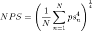
where  is the original power which is smoothed with a rolling window
and N is the total number of samples.
is the original power which is smoothed with a rolling window
and N is the total number of samples.
The function metrics.normalized_power_score allows to compute this
score:
>>> from skcycling.datasets import load_fit
>>> from skcycling.io import bikeread
>>> from skcycling.metrics import normalized_power_score
>>> ride = bikeread(load_fit()[0])
>>> mpa = 400
>>> np_score = normalized_power_score(ride['power'], mpa)
>>> print('Normalized power {:.2f} W'.format(np_score))
Normalized power 218.49 W
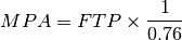
If you only have the functional threshold power, you need to first convert it to maximum power aerobic:
>>> from skcycling.metrics import ftp2mpa
>>> ftp = 304
>>> np_score = normalized_power_score(ride['power'], ftp2mpa(ftp))
>>> print('Normalized power {:.2f} W'.format(np_score))
Normalized power 218.49 W
Examples:
3.2.2. Intensity factor®
The intensity factor® [A2012] is defined as the normalized power® score normalized by the functional threshold power such as:

The function metrics.intensity_factor_score allows to compute this
metric:
>>> from skcycling.metrics import intensity_factor_score
>>> if_score = intensity_factor_score(ride['power'], mpa)
>>> print('Intensity factor {:.2f}'.format(if_score))
Intensity factor 0.72
Note that all our computation consider the maximum power aerobic for
consistency. If you only have the functional threshold power, use
metrics.ftp2mpa:
>>> if_score = intensity_factor_score(ride['power'], ftp2mpa(ftp))
>>> print('Intensity factor {:.2f}'.format(if_score))
Intensity factor 0.72
Examples:
3.2.3. Training stress score®
The training stress score® corresponds to the intensity factor® normalized by the time of the activity:
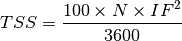
The function metrics.training_stress_score allows to compute this
score:
>>> from skcycling.metrics import training_stress_score
>>> ts_score = training_stress_score(ride['power'], mpa)
>>> print('Training stress score {:.2f}'.format(ts_score))
Training stress score 32.38
If you use the functional threshold metric, you need to convert it to the
maximum power aerobic using metrics.ftp2mpa:
>>> ts_score = training_stress_score(ride['power'], ftp2mpa(ftp))
>>> print('Training stress score {:.2f}'.format(ts_score))
Training stress score 32.38
Examples:
3.2.4. Training load score
Grappe et al. [G2009] compute the load of an activity as a weighted sum of the time spend in the different ESIE zones.
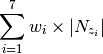
The function metrics.training_load_score compute this metric:
>>> from skcycling.metrics import training_load_score
>>> tl_score = training_load_score(ride['power'], mpa)
>>> print('Training load score {:.2f}'.format(tl_score))
Training load score 74.90
If you use the functional threshold metric, you need to convert it to the
maximum power aerobic using metrics.ftp2mpa:
>>> tl_score = training_load_score(ride['power'], ftp2mpa(ftp))
>>> print('Training load score {:.2f}'.format(tl_score))
Training load score 74.90
Examples:
3.3. Cyclist record power-profile
The record power-profile is a data derivative computed from the power information of several file. It is used to assess the potential and performance of cyclist [P2011] and calibrate the training of cyclist.
Before to focus on the record power-profile and the facilities provided by
scikit-cycling to provide this analysis, we will first define how to compute
a power-profile.
3.3.1. Power-profile for a single activity
A power-profile is computed for an activity and it is computed by taking the
maximum power delivered for different amount of time (e.g. from 1 seconds to 3
hours). The function extraction.activity_power_profile computes this
profile for a given max duration:
>>> from skcycling.datasets import load_fit
>>> from skcycling.io import bikeread
>>> from skcycling.extraction import activity_power_profile
>>> ride = bikeread(load_fit()[0], drop_nan='columns')
>>> power_profile = activity_power_profile(ride, max_duration='00:08:00')
Examples:
3.3.2. Record power-profile
The record power-profile of a cyclist is computed by taking the maximum of the
all available power-profile of activities for the different duration. It would
be possible to concatenate all pandas Series returned by the function
extraction.activity_power_profile and create a pandas
DataFrame. However, it is quite tedious and scikit-learn solve this issue
with the class Rider.
Rider makes it possible to add and remove power-profile of activities
as well as compute record power-profile for a specific period of time during the
year:
>>> from skcycling import Rider
>>> rider = Rider()
>>> rider.add_activities(load_fit())
Once, the power-profile for each activity is added, they can be accessed via the attributes rider.power_profile_ which is a pandas DataFrame:
>>> print(rider.power_profile_.head())
                  2014-05-07 12:26:22  2014-05-11 09:39:38  \
cadence 00:00:01            78.000...           100.000...
        00:00:02            64.000...            89.000...
        00:00:03            62.666...            68.333...
        00:00:04            62.500...            59.500...
        00:00:05            64.400...            63.200...

                  2014-07-26 16:50:56
cadence 00:00:01            60.000...
        00:00:02            58.000...
        00:00:03            56.333...
        00:00:04            59.250...
        00:00:05            61.000...
The record power-profile is computed such as:
>>> record_power_profile = rider.record_power_profile()
Note that record_power_profile accepts two parameters range_dates and
columns which limit to some dates or type of data the computation of the
record.
Examples:
3.3.3. Store and load power-profile for a rider
The methods to_csv and from_csv allows to store and load a cyclist
power-profile.
Examples:
3.4. Determination of the Maximum Power Aerobic
Using the record power-profile, Pinot et al. proposes a method to estimate the
Maximum Power Aerobic [P2014]. The function metrics.aerobic_meta_model
implements the algorithm:
>>> from skcycling.metrics import aerobic_meta_model
>>> mpa, t_mpa, aei, _, _ = aerobic_meta_model(rider.record_power_profile())
References
| [P2011] | Pinot, J., and F. Grappe. “The record power profile to assess performance in elite cyclists.” International journal of sports medicine 32.11 (2011): 839-844. |
| [P2014] | Pinot, J., and F. Grappe. “Determination of Maximal Aerobic Power from the Record Power Profile to improve cycling training.” Journal of Science and Cycling 3.1 (2014): 26. |
| [G2009] | (1, 2, 3, 4) Grappe, F. “Cyclisme et optimisation de la performance: science et méthodologie de l’entraînement.” De Boeck Supérieur, 2009. |
| [A2012] | (1, 2, 3, 4, 5) Allen, H., and A. Coggan. “Training and racing with a power meter.” VeloPress, 2012. |
Notes
Normalized Power® (NP), Intensity Factor® (IF), and Training Stress Score® (TSS) are registered trademarks of Peaksware, LLC.