Compute Power-Profile for an Activity

This example shows how to compute the power-profile of a cyclist for a single activity. We will also show how to plot those information.

# Authors: Guillaume Lemaitre <g.lemaitre58@gmail.com>
# License: BSD 3 clause

print(__doc__)

First, we will load an activity from the toy data set available in scikit-cycling.

from skcycling.datasets import load_fit
from skcycling.io import bikeread

ride = bikeread(load_fit()[0], drop_nan='columns')

We will only select some of interesting information

columns_selected = ['power', 'speed', 'cadence']
ride = ride[columns_selected]

The power-profile is extracted from the ride. By default, the maximum duration corresponds to the duration of the ride. However, to limit the processing, we limit the extraction to 8 minutes.

from skcycling.extraction import activity_power_profile

power_profile = activity_power_profile(ride, '00:08:00')
print('The power-profile is:\n {}'.format(power_profile))

Out:

The power-profile is:
 cadence  00:00:01    78.000000
         00:00:02    64.000000
         00:00:03    62.666667
         00:00:04    62.500000
         00:00:05    64.400000
         00:00:06    64.500000
         00:00:07    64.571429
         00:00:08    64.625000
         00:00:09    64.222222
         00:00:10    62.000000
         00:00:11    61.909091
         00:00:12    62.083333
         00:00:13    61.846154
         00:00:14    64.928571
         00:00:15    60.466667
         00:00:16    65.437500
         00:00:17    66.000000
         00:00:18    65.888889
         00:00:19    65.842105
         00:00:20    65.550000
         00:00:21    66.000000
         00:00:22    66.136364
         00:00:23    66.391304
         00:00:24    66.625000
         00:00:25    66.960000
         00:00:26    67.307692
         00:00:27    67.666667
         00:00:28    67.964286
         00:00:29    68.103448
         00:00:30    68.233333
                       ...
speed    00:07:30     7.607184
         00:07:31     7.610104
         00:07:32     7.624642
         00:07:33     7.627801
         00:07:34     7.631033
         00:07:35     7.967097
         00:07:36     7.971888
         00:07:37     7.976606
         00:07:38     7.981303
         00:07:39     7.986033
         00:07:40     7.990848
         00:07:41     7.995642
         00:07:42     8.000258
         00:07:43     8.005011
         00:07:44     8.009690
         00:07:45     8.014245
         00:07:46     8.019255
         00:07:47     8.024086
         00:07:48     8.029380
         00:07:49     8.034599
         00:07:50     8.039849
         00:07:51     8.045524
         00:07:52     7.591794
         00:07:53     7.591892
         00:07:54     7.591876
         00:07:55     7.591501
         00:07:56     7.603939
         00:07:57     7.616686
         00:07:58     7.629561
         00:07:59     7.642568
Name: 2014-05-07 12:26:22, Length: 1437, dtype: float64

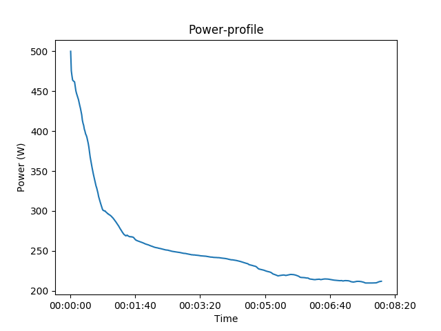
The power_profile is a pandas Series with multi-index. The additional information (e.g. speed, cadence, etc.) associated with the maximum power extracted are also computed. It is possible to plot those information using pandas. For instance, we will plot only the power information.

import matplotlib.pyplot as plt

power_profile.loc['power'].plot(title='Power-profile')
plt.xlabel('Time')
plt.ylabel('Power (W)')

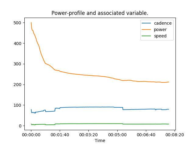
In the same manner, we could plot all information using the pandas API.

power_profile.unstack().T.plot(title='Power-profile and associated variable.')
plt.xlabel('Time')

plt.show()

Total running time of the script: ( 0 minutes 1.171 seconds)