Compute a record power profile
This example illustrates the usage of skcycling.Rider to compute
easily record power-profile,
print(__doc__)

# Authors: Guillaume Lemaitre <g.lemaitre58@gmail.com>
# License: BSD 3 clause
We will use the skcycling.Rider class to compute power-profile for
the toy data sets.
Out:
The computed activities are:
                   2014-05-07 12:26:22  2014-05-11 09:39:38  \
cadence 00:00:01            78.000000           100.000000
        00:00:02            64.000000            89.000000
        00:00:03            62.666667            68.333333
        00:00:04            62.500000            59.500000
        00:00:05            64.400000            63.200000
        00:00:06            64.500000            66.500000
        00:00:07            64.571429            69.285714
        00:00:08            64.625000            71.875000
        00:00:09            64.222222            67.888889
        00:00:10            62.000000            76.800000
        00:00:11            61.909091            73.090909
        00:00:12            62.083333            75.333333
        00:00:13            61.846154            70.769231
        00:00:14            64.928571            73.142857
        00:00:15            60.466667            75.400000
        00:00:16            65.437500            82.562500
        00:00:17            66.000000            78.647059
        00:00:18            65.888889            79.666667
        00:00:19            65.842105            80.473684
        00:00:20            65.550000            81.250000
        00:00:21            66.000000            81.952381
        00:00:22            66.136364            82.727273
        00:00:23            66.391304            83.391304
        00:00:24            66.625000            84.000000
        00:00:25            66.960000            84.560000
        00:00:26            67.307692            85.153846
        00:00:27            67.666667            85.740741
        00:00:28            67.964286            86.214286
        00:00:29            68.103448            86.689655
        00:00:30            68.233333            87.133333
...                               ...                  ...
speed   01:51:14                  NaN                  NaN
        01:51:15                  NaN                  NaN
        01:51:16                  NaN                  NaN
        01:51:17                  NaN                  NaN
        01:51:18                  NaN                  NaN
        01:51:19                  NaN                  NaN
        01:51:20                  NaN                  NaN
        01:51:21                  NaN                  NaN
        01:51:22                  NaN                  NaN
        01:51:23                  NaN                  NaN
        01:51:24                  NaN                  NaN
        01:51:25                  NaN                  NaN
        01:51:26                  NaN                  NaN
        01:51:27                  NaN                  NaN
        01:51:28                  NaN                  NaN
        01:51:29                  NaN                  NaN
        01:51:30                  NaN                  NaN
        01:51:31                  NaN                  NaN
        01:51:32                  NaN                  NaN
        01:51:33                  NaN                  NaN
        01:51:34                  NaN                  NaN
        01:51:35                  NaN                  NaN
        01:51:36                  NaN                  NaN
        01:51:37                  NaN                  NaN
        01:51:38                  NaN                  NaN
        01:51:39                  NaN                  NaN
        01:51:40                  NaN                  NaN
        01:51:41                  NaN                  NaN
        01:51:42                  NaN                  NaN
        01:51:43                  NaN                  NaN

                  2014-07-26 16:50:56
cadence 00:00:01            60.000000
        00:00:02            58.000000
        00:00:03            56.333333
        00:00:04            59.250000
        00:00:05            61.000000
        00:00:06            62.333333
        00:00:07            63.571429
        00:00:08            63.750000
        00:00:09            63.444444
        00:00:10            63.000000
        00:00:11            62.363636
        00:00:12            61.916667
        00:00:13            62.076923
        00:00:14            62.642857
        00:00:15            63.400000
        00:00:16            62.625000
        00:00:17            61.823529
        00:00:18            61.109223
        00:00:19            60.468319
        00:00:20            59.889806
        00:00:21            59.364771
        00:00:22            58.885922
        00:00:23            58.447235
        00:00:24            58.043689
        00:00:25            57.671068
        00:00:26            57.325803
        00:00:27            57.004854
        00:00:28            56.705617
        00:00:29            56.425845
        00:00:30            68.500000
...                               ...
speed   01:51:14             5.478008
        01:51:15             5.478270
        01:51:16             5.478586
        01:51:17             5.478993
        01:51:18             5.479495
        01:51:19             5.480122
        01:51:20             5.480738
        01:51:21             5.481302
        01:51:22             5.481879
        01:51:23             5.482435
        01:51:24             5.482988
        01:51:25             5.483579
        01:51:26             5.484132
        01:51:27             5.484607
        01:51:28             5.485022
        01:51:29             5.485448
        01:51:30             5.485894
        01:51:31             5.486276
        01:51:32             5.486645
        01:51:33             5.486973
        01:51:34             5.487264
        01:51:35             5.487511
        01:51:36             5.487729
        01:51:37             5.487925
        01:51:38             5.488108
        01:51:39             5.488282
        01:51:40             5.488451
        01:51:41             5.488631
        01:51:42             5.488807
        01:51:43             5.488291

[40218 rows x 3 columns]
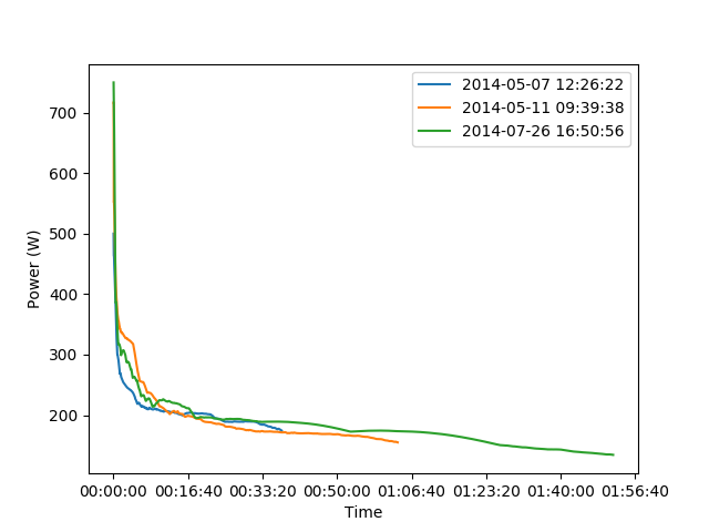
The different power-profile for the activities can be plotted as follow
import matplotlib.pyplot as plt

rider.power_profile_.loc['power'].plot()
plt.xlabel('Time')
plt.ylabel('Power (W)')
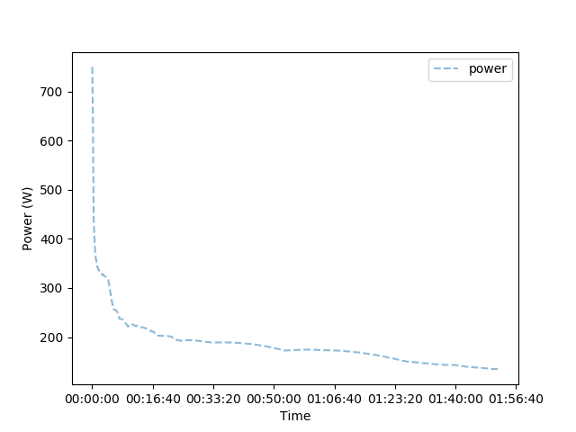
Once that the power-profile for each activity are computed, we can compute the record power-profile for the rider and plot it.
rider.record_power_profile()['power'].plot(alpha=0.5,
                                           style='--',
                                           legend=True)
plt.xlabel('Time')
plt.ylabel('Power (W)')

plt.show()
Total running time of the script: ( 0 minutes 26.851 seconds)