Plot Activity Data

This example shows how to plot the information read with the function skcycling.io.bikeread using pandas.

# Authors: Guillaume Lemaitre <g.lemaitre58@gmail.com>
# License: BSD 3 clause

print(__doc__)

scikit-cycling has couple of fit files stored which can be used as toy data.

from skcycling.datasets import load_fit

filename_fit = load_fit()[0]  # catch the first toy file
print('The fit file which will be used is stored at: \n {}'
      .format(filename_fit))

Out:

The fit file which will be used is stored at:
 /home/docs/checkouts/readthedocs.org/user_builds/scikit-cycling/envs/stable/local/lib/python2.7/site-packages/skcycling/datasets/data/2014-05-07-14-26-22.fit

The function skcycling.io.bikeread allows to read the file without any extra information regarding the format.

from skcycling.io import bikeread

ride = bikeread(filename_fit, drop_nan='columns')
print('The ride is the following:\n {}'.format(ride.head()))

Out:

The ride is the following:
                      elevation  cadence  distance  power  speed
2014-05-07 12:26:22       64.8     45.0      3.05  256.0  3.036
2014-05-07 12:26:23       64.8     42.0      6.09  185.0  3.053
2014-05-07 12:26:24       64.8     44.0      9.09  343.0  3.004
2014-05-07 12:26:25       64.8     45.0     11.94  344.0  2.846
2014-05-07 12:26:26       65.8     48.0     15.03  389.0  3.088

First, we can list the type of data available in the DataFrame

print('The available data are {}'.format(ride.columns))

Out:

The available data are Index([u'elevation', u'cadence', u'distance', u'power', u'speed'], dtype='object')

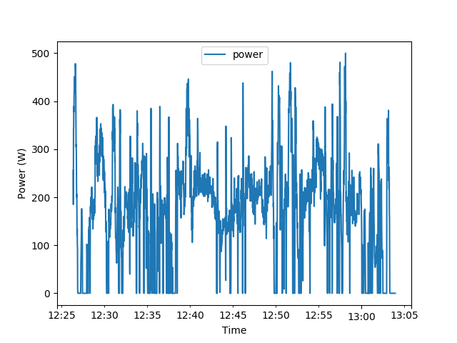
Plotting a specific column (e.g. power) is easy using the pandas plot function.

import matplotlib.pyplot as plt

ride['power'].plot(legend=True)
plt.xlabel('Time')
plt.ylabel('Power (W)')

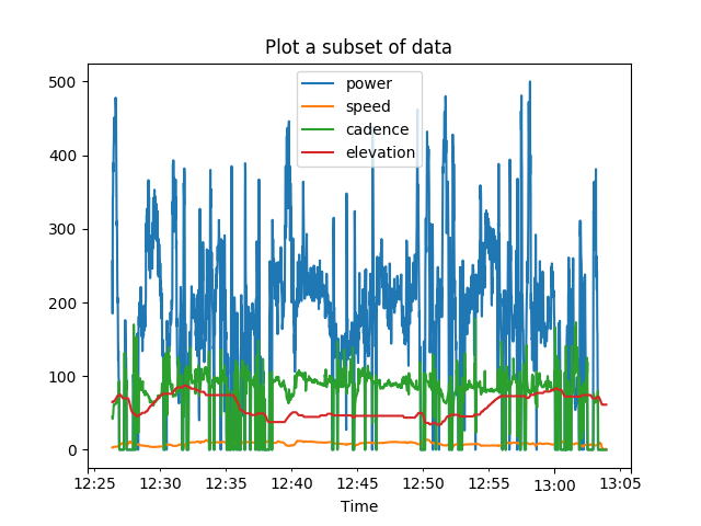
In the same manner we can plot several column at the same time.

columns = ['power', 'speed', 'cadence', 'elevation']
ride[columns].plot(legend=True)
plt.xlabel('Time')
plt.title('Plot a subset of data')

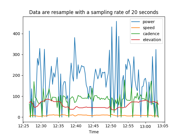
To smooth the data, we can even resample them before to plot them

ride[columns].resample('20S').interpolate().plot(legend=True)
plt.xlabel('Time')
plt.title('Data are resample with a sampling rate of 20 seconds')

plt.show()

Total running time of the script: ( 0 minutes 1.287 seconds)